The regulatory interactions between genes are identified using two scores: R1 and R2.
The regulatory relation between two genes is first evaluated using R1(X; Y; i; p) in Equation 1. R1 represents the correlation
between gene X at time point i and gene Y at time point i + p. p is the time span of the gene regulation.
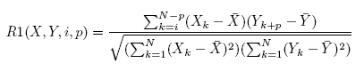 [Equation (1) for the R1 score] [Equation (1) for the R1 score]In Equation 1, N is the total number of time points contained in the time span, Xk and Yk are the
expression levels of genes X and Y at time k, and X and Y are the average gene expression levels at all time
points of the time span. Among the total i X p candidate regulations, the regulation with the maximum
absolute value of R1(X; Y; i; p) is selected as the regulatory relation between genes X and Y .
The R1 score of each gene regulation is iteratively calculated using Algorithm 1. For genes A and B, the regulation with the largest absolute R1 score is chosen for the regulation between the genes and represented as R1(A; B; t1; p) with t2 = t1 + p.
After we construct a regulation list, we compute the R2 score for the gene pairs in the regulation list to distinguish the gene regulatory relations with the same correlation but different gene expression levels. R2 is basically the Euclidean distance of the expression levels of the two genes.
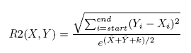 where, where, 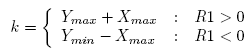 [Equation (2) for the R2 score] [Equation (2) for the R2 score]
In Equation 2, X and Y are the average gene expression levels at all time points in the time span. Xmax is
the maximum gene expression value of gene X. Ymax and Ymin are the maximum and minimum gene
expression value of gene Y , respectively.
When computing the R2 score in a time span, the time span is divided into smaller sub-timespans as
follows. The R2 score is not computed for sub-timespans with less than 6 time points.
1. A time point with the minimum expression level of the regulator gene becomes a splitting point of
the time span.
2. Each sub-timespan starts with at least 3 consecutive time points that have a positive slope of a curve
representing gene expression levels, and ends with at least 3 consecutive time points with a negative
slope.
3. Each sub-timespan encompasses at least 6 time points, including the start and ending time points.
|